If you haven’t seen a Skew-T chart before, to say they can look a little intimidating is a huge understatement. But with a little practice, you can become a Skew-T master and open up new doors to learn about a variety of meteorological subjects. Skew-T charts are incredibly useful for quickly and accurately viewing the structure of the atmosphere all the way from the surface to 100,000 feet, and they’ve been around for a LONG time – since 1947, to be exact1.
Skew-T charts are most commonly used to plot parameters measured by radiosondes as they rise throughout the atmosphere. They only plot three measurements: temperature, dew point, and wind velocity (the speed AND direction of the wind). Additionally, there are 5 lines on a Skew-T: isotherms, isobars, dry adiabats, moist adiabats, and saturation mixing ratio lines.
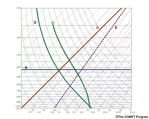
Isobars (A), dry adiabats (B), moist adiabats (C), isotherms (D), and saturation mixing ratio lines.
Credit: UCAR MetEd module on reading Skew-T charts. If you are looking for more information, I suggest you try the module! You will need to register to join, but registration is free,
Besides simply acting as a template to plot the temperature, dewpoint, and wind, Skew-Ts are useful for easily finding the locations and values of important levels and parameters of the atmosphere. CAPE, the LCL, and the LFC are just a few things that can easily be found with a Skew-T.
Let’s start our journey by learning about each line on a Skew-T.
Isotherms

Credit: UCAR Comet Program Skew-T module
Isotherms are lines of constant temperature. They are the namesake of the Skew-T chart because they are skewed 45 degrees to the right. Skewing the Ts may seem a little unintuitive, but a Skew-T allows us to easily calculate important atmospheric levels and parameters like the Lifting Condensation Level (LCL), Level of Free Convection (LFC), the Equilibrium Level, and CAPE. A Stüve is like a Skew-T but without the skewed temperature lines. It is not as useful for most meteorological applications because the adiabats on it are not curved, meaning we can’t accurately calculate the things listed above.
Isobars

Credit: UCAR Comet Program Skew-T module
Isobars are defined as “lines of constant pressure.” On a Skew-T chart, pressure, NOT height, is plotted on the y-axis, so isobars are simply parallel to the x-axis. Because pressure decreases more slowly with height the higher you go, pressure is plotted in a logarithmic fashion on Skew-T charts. For this reason, Skew-T charts are also commonly called Skew-T/Log-P charts. If we didn’t plot pressure in logarithms, the Skew-T charts would be as high as the weather balloons they plot traveled – approximately 100,000 feet high!
Dry Adiabats

Credit: UCAR Comet Program Skew-T module
Adiabatic processes are processes in which no heat is exchanged with the outside system (in our case, the atmosphere), and dry adiabats show how much an unsaturated parcel cools when lifted through the atmosphere. You are probably thinking “how can a parcel cool and maintain the same heat content?” Well, keep in mind that as an air parcel rises, it expands due to the surrounding atmosphere exerting less pressure on it, so the total heat content remains the same.
Adiabatic processes are a consequence of the First Law of Thermodynamics, which states that the heat added to a certain mass of a gas is equal to its change in internal energy + the work done BY the gas ON the environment. My doing some nifty mathematical maneuvering and applying the ideal gas law, we find that the first law states that changes in temperature are positively correlated with changes in pressure. I’ll discuss this and more in a tutorial in the future, but the important thing to know is that when an unsaturated air parcel rises and ANY air parcel sinks, it will travel parallel to these adiabats.
These adiabats follow the “Dry Adiabatic Lapse Rate,” which is approximately 10 degrees Celsius per kilometer.
Moist Adiabats

Credit: UCAR Comet Program Skew-T module
When saturated air rises, it follows the “saturation” or “moist adiabats.” When air reaches saturation, gaseous water vapor condenses into liquid water droplets, and this phase change releases “latent heat” into the atmosphere. Because of this, the moist adiabatic lapse rate is ALWAYS less than the dry adiabatic lapse rate, but as you can see above, moist adiabats are NOT parallel and vary quite a bit with both temperature AND altitude.
The most important thing to remember about moist adiabats is that a saturated air parcel will ONLY follow them if it is rising. If the parcel is sinking, it is warming away from saturation and will follow the dry adiabats.
Saturation Mixing Ratio Lines

Credit: UCAR Comet Program Skew-T module
The saturation mixing ratio is the ratio, in grams of water vapor per kilogram of air, that an air parcel must have at a given pressure and temperature to be considered “saturated.” Once an air parcel is saturated, it generally cannot hold any more water vapor.
Now that you know the lines – let’s find out how we can use them to calculate some particularly important levels of the atmosphere. We’ll learn how to calculate the lifting condensation level (LCL), the convective condensation level (CCL), the level of free convection (LFC), and the equilibrium level (EL), as well as convective available potential energy (CAPE) and convective inhibition (CIN).
Lifting Condensation Level (LCL)

Lifting Condensation Level
Credit: UCAR MetEd COMET Program
The LCL is the pressure level an air parcel would need to be raised (dry adiabatically) to to become saturated. To find the LCL, follow a dry adiabat from your surface environmental temperature and a saturation mixing ratio line from your surface dewpoint temperature. The intersection of these marks the location of the LCL. The LCL is important because it marks location where the air parcel stops rising at the dry adiabatic lapse rate and switches to the moist adiabatic lapse rate.
Convective Condensation Level (CCL)
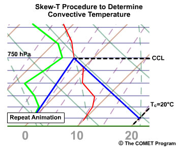
Convective Condensation Level. The Convective Temperature (Tc) can be found by taking a dry adiabat down from the CCL to the surface.
A closely related level is the Convective Condensation Level, or CCL. The CCL is the pressure level that a parcel, if heated to the “convective temperature,” would freely rise and form a cumulus cloud. The convective temperature is the temperature the surface must reach so that air can freely rise, and the CCL is at the intersection of the environmental temperature (NOT a dry adiabat from the surface… that’s the LCL) and the saturation mixing ratio line from the surface dewpoint temperature.
Notes: The LCL and CCL are useful for determining the height of cloud bases. For non-convective clouds that are forced to rise, the LCL is a good approximation. On the other hand, the CCL is a better estimate for clouds formed by convection, like cumulus clouds. In reality, cloud bases are generally somewhere between the LCL and CCL.
The reason why thunderstorms in the desert often have high bases is because surface dewpoints are low there, causing the LCL and CCL to be high in the atmosphere. Conversely, thunderstorms in humid locations generally have lower bases because the LCL is lower.
Level of Free Convection (LFC)
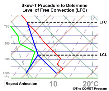
Level of free convection. It is calculated by taking a moist adiabat from the LCL until you intersect the environmental temperature.
The LFC is the pressure level an air parcel would need to be raised so that its temperature is equal with the environmental temperature. It is found by taking the moist adiabat from the LCL until it intersects the environmental temperature. After this, the air parcel is warmer than its environment and can freely rise (hence the name – level of free convection).
There are a few isolated situations where this approach won’t work – for example, if the surface has reached the “convective temperature” mentioned above, the LFC is at the surface. But for the vast majority of situations, this method works beautifully.
Not all soundings have an LFC. If the moist adiabat never intersects the environmental temperature because the atmosphere is relatively stable and does not exhibit a sharp decrease in temperature with height, there is no LFC. Additionally, many places that have an LFC during the day may not have one at night, when the surface is cooler and the atmosphere is more stable.
Equilibrium Level (EL)
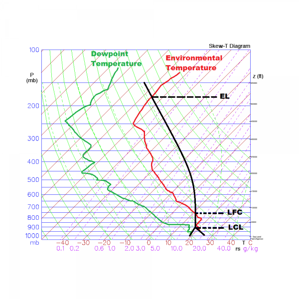
A Sample Skew-T Diagram. The slanted red lines are lines of constant temperature, the dotted purple lines are lines of constant mixing ratio, the solid curved green lines are dry adiabats, and the curved green lines are moist adiabats.
The Lifting Condensation Level (LCL), Level of Free Convection (LFC), and Equilibrium Level (EL) are labeled. The CAPE is bounded on the bottom by the LFC and the top by the EL and is the total area between the black line (path of the air parcel) and red line (environmental temperature).
Retrieved from Rebecca Ladd’s Weather Blog
The equilibrium level only exists if there is an LFC, and it is defined as the level at which the moist adiabat denoting the parcel’s path recrosses the environmental temperature. At the EL, the air parcel is the same temperature as its environment, and above it, it is cooler and more dense. The EL can be found by looking at the “anvils” on thunderstorms, as these mark the location where a rising air parcel is no longer positively buoyant. The “overshooting top” of a thunderstorm exceeds the equilibrium level, but this is only because the momentum of the storm’s uber-powerful updraft is allowing it to reach a higher altitude, NOT because the air above the equilibrium level is positively buoyant.
Convective Available Potential Energy (CAPE) and Convective Inhibition (CIN)

Sounding showing CIN and CAPE
Credit: UCAR
CAPE is the area bounded by the environmental temperature and the temperature of a parcel as it rises along the moist adiabatic lapse rate. By definition, the lower bound of the CAPE is the LFC, and the upper bound is the EL. Because CAPE measures how buoyant an air parcel is relative to its environment, it can be used to estimate the maximum strength of updrafts in a storm, and by association, how severe a storm can become. If you want big storms, you need big CAPE. Period.
CIN is CAPE’s antithesis: while CAPE measures positive buoyancy and the strength of convection possible, CIN measures negative buoyancy and the resistance to convection. CIN is bounded by the environmental temperature on the right and the temperature of the rising parcel on the right, and is measured from the LFC down to wherever the temperature of the environment and temperature of the parcel are the same, which is almost always the surface. In this area, the temperature of the parcel is less than the environment, thus rendering the parcel more dense and causing it to sink in the absence of any external forcing. CIN generally peaks during the early morning and decreases during the day as the sun heats the surface.
CIN is actually a necessary ingredient for severe storms because it allows CAPE to build to tremendous levels by preventing convection and mixing of the atmosphere during the morning hours. When heating from the surface finally erodes the CIN, CAPE values have grown astronomically large and any storm development is explosive, leading to powerful supercells with large hail, damaging winds, and tornadoes.
Here’s a classic severe weather sounding from Oklahoma City that was taken 3 hours before the devastating 2013 Moore, OK EF-5 tornado. See if you can find the LCL, CCL, LFC, EL, CAPE, and CIN on this sounding!
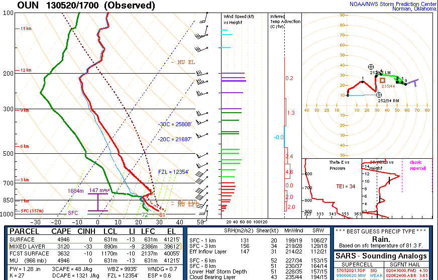
A CLASSIC severe weather sounding, with a pronounced “capping inversion” (CIN) that keeps convection from gradually occurring throughout the day, allowing it to explode all at once in the late afternoon/evening hours when the cap breaks. There is also a ton of CAPE and strong wind shear throughout the atmosphere. The 2013 Moore EF-5 tornado touched down 3 hours after this sounding was taken.
Retrieved from Rebecca Ladd’s Weather Blog
Thanks for reading, I hope you learned something!
Written by Charlie Phillips – charlie.weathertogether.net. Last updated 5/17/2017
References:
- National Weather Service (n.d.). Skew-T Log-P Diagrams. Retrieved May 10, 2017, from http://www.srh.noaa.gov/jetstream/upperair/skewt.html
- University Corporation for Atmospheric Research (n.d.). Skew-T Mastery. Retrieved May 17, 2017, from http://www.meted.ucar.edu/mesoprim/skewt/
- Ladd, R. (2014, April 25). The Basics of a severe weather sounding. Retrieved May 17, 2017, from http://wx4cast.blogspot.com/2014/04/the-basics-of-severe-weather-sounding.html